Molecular Dynamics Simulation

DFTpy performs molecular dynamics (MD) simulations with ASE_. This is one example to run NVT (canonical ensemble) simulation:

The output md.traj can be converted with ASE_:

Run this cell to install DFTpy in google colab

!python -m pip install "git+https://github.com/Quantum-MultiScale/DFTpy.git@dev"

Download the pseudopotential file

!wget https://raw.githubusercontent.com/Quantum-MultiScale/DFTpy/dev/DATA/Al_lda.oe01.recpot

import os
import pathlib
import numpy as np
from ase.lattice.cubic import FaceCenteredCubic
from ase.md.langevin import Langevin
from ase.md.verlet import VelocityVerlet
from ase.md.velocitydistribution import MaxwellBoltzmannDistribution
from ase.io.trajectory import Trajectory
from ase import units
from ase.md.npt import NPT

from dftpy.config import DefaultOption, OptionFormat
from dftpy.interface import OptimizeDensityConf
from dftpy.api.api4ase import DFTpyCalculator

For parallel implementation when running in python

# MPI / parallel setup
from dftpy.mpi import MP, sprint
mp = MP(parallel=False) # Set parallel=True to run in parallel

Define initial configuration with DFTpy

conf = DefaultOption()
conf['PATH']['pppath'] = '../DATA'
conf['PP']['Al'] = 'Al_lda.oe01.recpot'
conf['OPT']['method'] = 'TN'
conf['KEDF']['kedf'] = 'WT'
conf['JOB']['calctype'] = 'Energy Force'
conf = OptionFormat(conf)

Build the system with ASE

size = 3
a = 4.24068463425528
T = 1023  # Kelvin
T *= units.kB
atoms = FaceCenteredCubic(directions=[[1, 0, 0], [0, 1, 0], [0, 0, 1]],
                          latticeconstant = a,
                          symbol="Al",
                          size=(size, size, size),
                          pbc=True)

Set the DFTpy calculator to the ase atoms

calc = DFTpyCalculator(config = conf) # DFTpy can be run in parallel using the MPI interface, as follows: DFTpyCalculator(config = conf, mp=mp)
atoms.calc = calc

Perform the dynamics

MaxwellBoltzmannDistribution(atoms, T, force_temp = True)

dyn = Langevin(atoms, 2 * units.fs, T, 0.1)

step = 0
interval = 1
def printenergy(a=atoms):
    global step, interval
    epot = a.get_potential_energy() / len(a)
    ekin = a.get_kinetic_energy() / len(a)
    print('Step={:<8d} Epot={:.5f} Ekin={:.5f} T={:.3f} Etot={:.5f}'.format(step, epot, ekin, ekin / (1.5 * units.kB), epot + ekin))
    step += interval

dyn.attach(printenergy, interval=1)

traj = Trajectory('md.traj', 'w', atoms)
dyn.attach(traj.write, interval=5)

dyn.run(500)

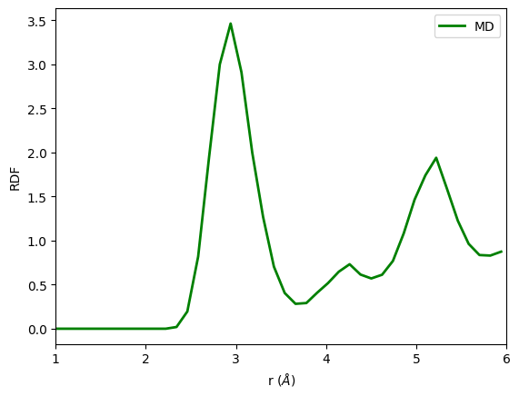
Analyse the trajectory by plotting the rdial distribution function (RDF)

from ase.geometry.analysis import Analysis
analysis = Analysis(list(Trajectory('md.traj')))
rdf = analysis.get_rdf(rmax=6, nbins=50, return_dists=True)
rdf = np.asarray(rdf).mean(axis=0)

import matplotlib.pyplot as plt

plt.plot(rdf[1], rdf[0], 'g', lw=2,label='MD')
plt.ylabel('RDF')
plt.xlabel(r'r ($\AA$)')
plt.xlim(1,6)
plt.legend()

<matplotlib.legend.Legend at 0x122f91f30>